Hands-on Exercise with QGIS¶

Now that you are aware of all the necessay background information, it is time to do work with the Milan case study. To asses differences in the average air temperature within different LCZ, you will perform the following steps:

download in your home folder the raw air temperature data from the C3S CDS in netCDF format and the LCZ map for Milan.

open and manipulate the netCDF in QGIS to obtain an analysis-ready raster layer containg the average air temperature for a given time period.

open the LCZ map in QGIS and perform raster layer zonal statistics to compute the average air temperature within each LCZ class

plot and compare the averages using statistical graphs

Materials¶

Data specification and software tools that you will use for the analysis are reported below.

LCZ map¶

The LCZ raster map of Milan you will use in the exercise has been derived by [4] and [5] from a Sentinel-2 image acquired in summer 2016. The map includes the subset of LCZ characterizing the Milan area. Some of the contiguous classes have been aggregated (as shown in the table below) with the purpose of obtaining zones with marked differences in the urban land-use features thus easing their comparison in terms of air temperature. In practice, contiguous LCZ classes may be more easily confused during the classification procedure and, in turn, differences in their contributions to air temperature may be biased or difficult to distinguish.

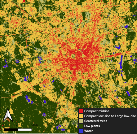
LCZ map of Milan

Raster Value	Description
1	Compact midrise
2	Compact low-rise, Open midrise, Open low-rise, Large low-rise
3	Scattered trees
4	Low plants
5	Water

The LCZ map of Milan (s2_lcz_milan.tif) (reference system: WGS84/UTM32N | EPSG:32632) in GeoTIFF format together with its predfined QGIS Style File (s2_lcz_milan.qml) can be download here.

Tip

Keep in the same folder both the raster map and its predefined QGIS style file to allow QGIS to automatically style the map when imported in a project.

Air temperature data¶

Air temperature data at a city level are included in the Climate variables for cities in Europe from 2008 to 2017 of the C3S CDS, which contains air temperature, specific humidity, relative humidity and wind speed for 100 European cities for the current climate. The variables are provided as netCDF files with an hourly temporal resolution on a 100m x 100 m spatial grid (reference system: ETRS89/LAEA Europe | EPSG: 3035).

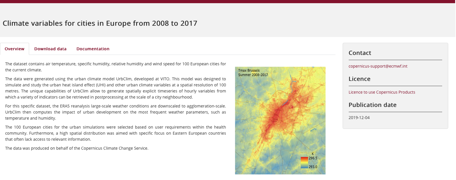
Climate variables for cities in Europe from 2008 to 2017 (https://cds.climate.copernicus.eu/cdsapp#!/dataset/sis-urban-climate-cities)

After register and login to the C3S CDS web portal, you have to download Milan data by specifying the variable of interest together with a time period (year and month). The selected data can be then downloaded as a .zip or .tar file. For this exercise you have to specify the following options before the download:

Variable = Air temperature

City = Milan

Year = 2016

Month = July

Format = Zip file (.zip)

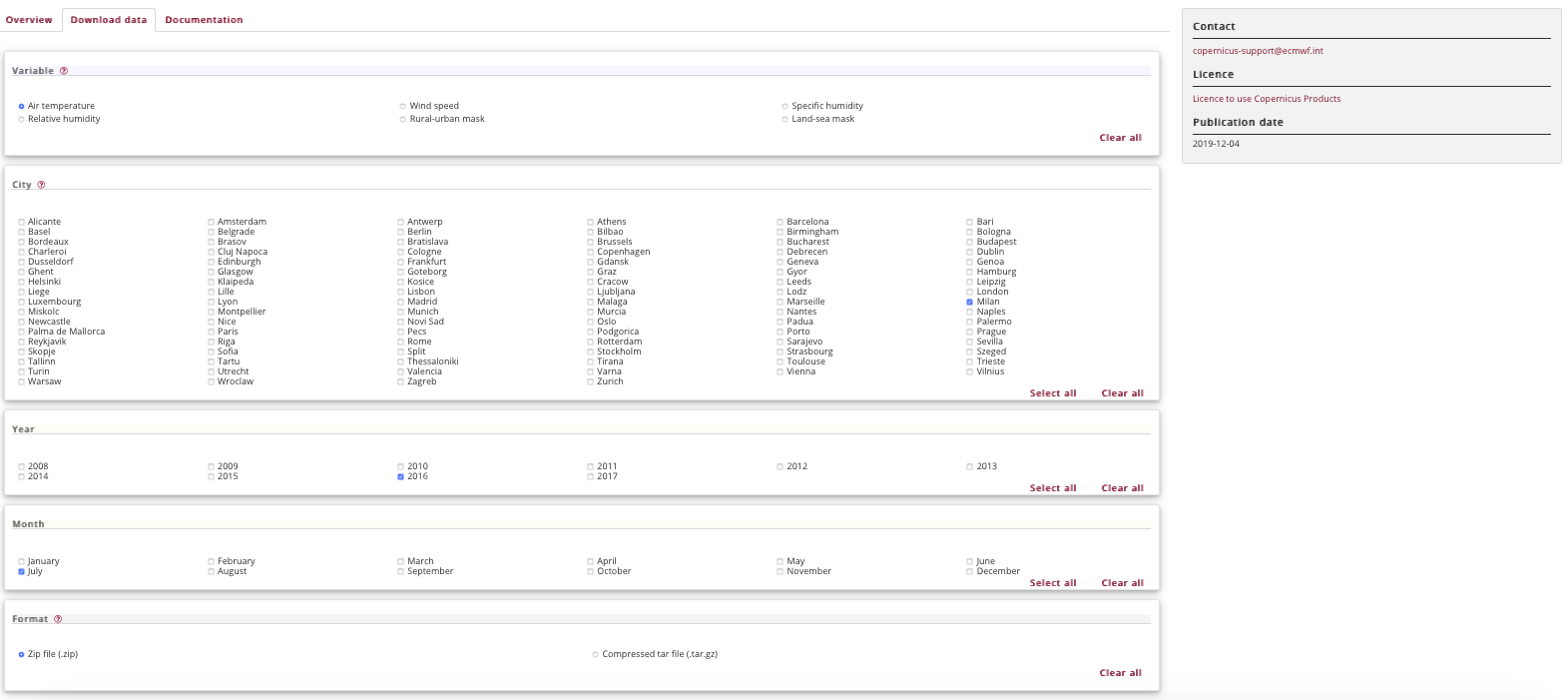
C3S CDS download page

The netCDF file is structured as a multidimensional spatial grid where each layer includes air temperature observations over Milan area at each time step (hour) in July 2016.

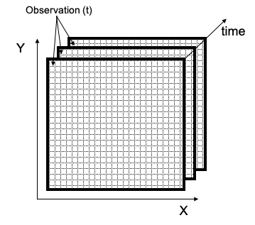
Schematic of the netCDF structure

Note

The original name of the downloaded file should be “tas_Milan_UrbClim_2016_07_v1.0.nc”

Software tools¶

To perform the exercise you will use QGIS . However, advance raster processing functionalities are not directly available within the QGIS core algorithms. To that end, you will use third-party algorithms from GRASS GIS which are integrated into the QGIS Processing Toolbox and they can be run directly from the QGIS interface.

Tip

GRASS GIS Loading

If you don’t see GRASS in the Processing Toolbox, verify in: Settings –> Options –> Processing –> Providers if GRASS provider is activated. GRASS system paths should be already set up if using macOS or Windows.

Data Processing¶

netCDF preprocessing¶

Open a new QGIS project and import as a raster layer (Layer –> Add Layer –> Add Raster Layer) the air temperature netCDF (tas_Milan_UrbClim_2016_07_v1.0.nc). The layer is imported as a multiband raster in which each band contains the hourly observation of air temperature over Milan (n. of bands = 744). In the following steps, you will manipulate the raster file obtained from the netCDF by projecting it to WGS84/UTM32N | EPSG:32632 and computing the averages of all bands.
Do Right Click on the layer name in the QGIS Layer Panel and then: Export –> Save As… to save the layer in GeoTIFF format by assigning its native reference system (ETRS89/LAEA Europe | EPSG: 3035).

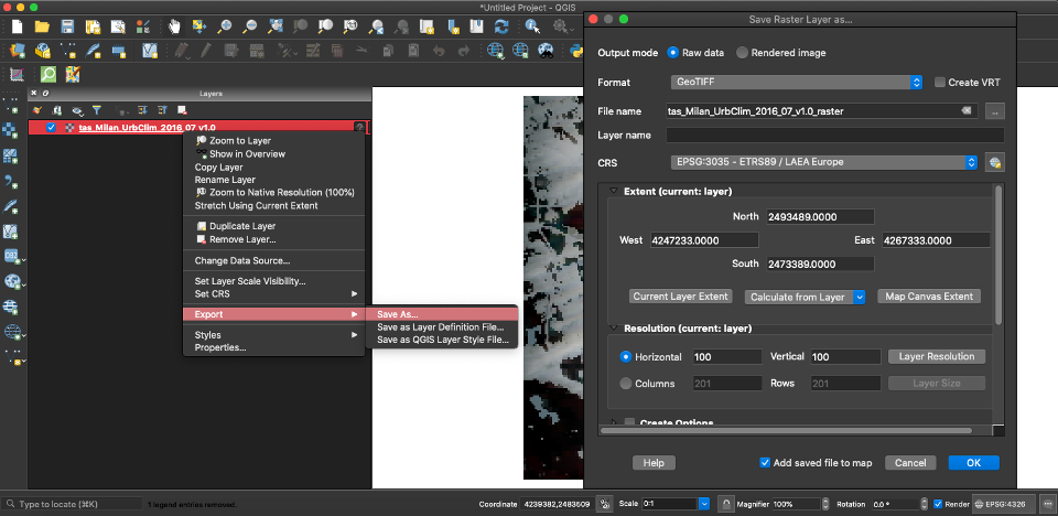
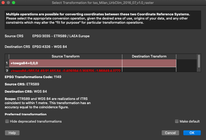
Accept the default coordinates conversion procedure suggested by QGIS by clicking Ok.

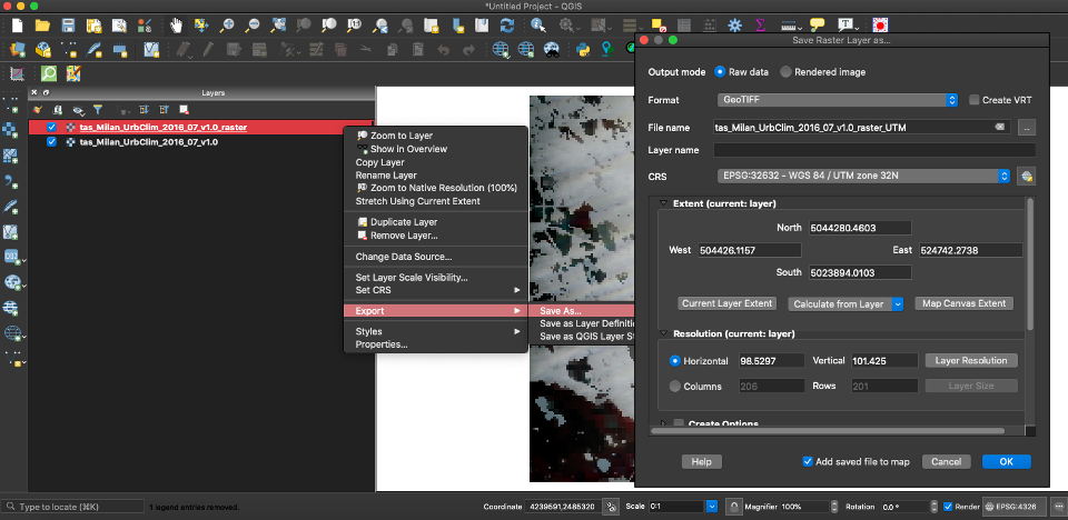
Create a second copy of the raster layer to assign the same projected reference system of the LCZ map (WGS84/UTM32N | EPSG:32632) by following the procedure explained in the previous step.

Tip

In case of issues with the presented procedure, you can directly download the projected raster layer from the above step.

Now, you have obtained a multiband raster layer projected to the same reference system of the LCZ map. The last step consists of computing the average air temperature in July 2016 at each pixel of the grid.

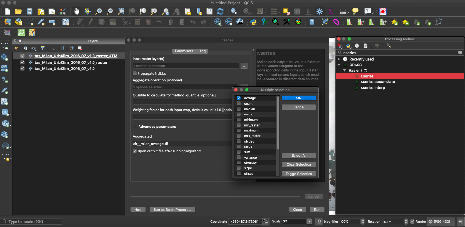
From the QGIS menu, open: Processing –> Toolbox and search for the GRASS GIS algorithm r.series which allows making each output cell value a function (e.g. the average) of the values assigned to the corresponding cells in the input list of raster bands or layers.
Run the algorithm on the projected multiband raster layer by specifying Average in the Aggregate operation tab to obtain the single-band raster of the average air temperature [K] for Milan in July 2016.

Warning

If you use QGIS on Windows, you have to set also the raster values range. In the r.series panel, open: Advanced Parameters –> Ignore values outside this range (lo,hi), set e.g. Min = -1000 and Max = 1000.

Tip

Name the output file as “air_t_milan_average”. The period (“.”) in the original name of the netCDF file may not be accepted by GRASS GIS as part of the output file name. In case of issues with the presented procedure, you can directly download the average air temperature raster.

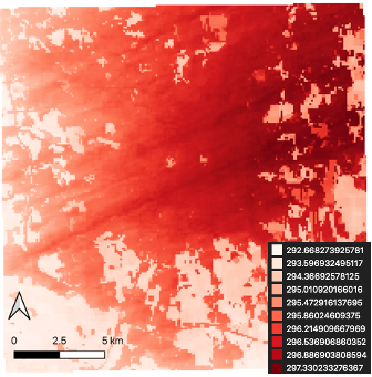
Single band raster of the average air temperature [K] for Milan in July 2016

Raster zonal statistics¶

To assess differences in the average air temperature within different LCZ, you need to compute raster statistics by class using the single band raster of the average air temperature for Milan in July 2016 and the LCZ map.

Open a new QGIS project and import the requested raster maps (air_t_milan_average.tif and s2_lcz_milan.tif).
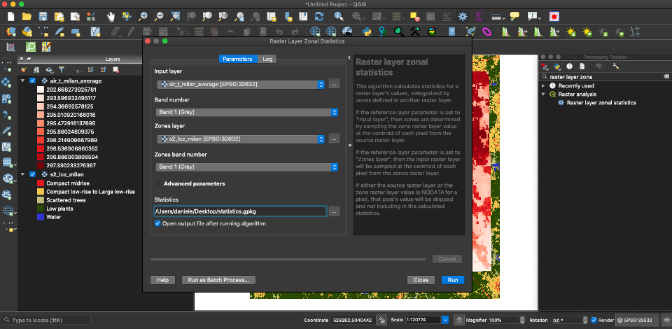
From the QGIS menu, open: Processing –> Toolbox and search for the QGIS algorithm Raster layer zonal statistics which allows you computing statistics for a raster layer’s values, categorized by zones defined in another raster layer. Specify as Input layer the average air temperature raster and as Zones layer the LCZ map. Save the output as a Shapefile or GeoPackage table.

Note

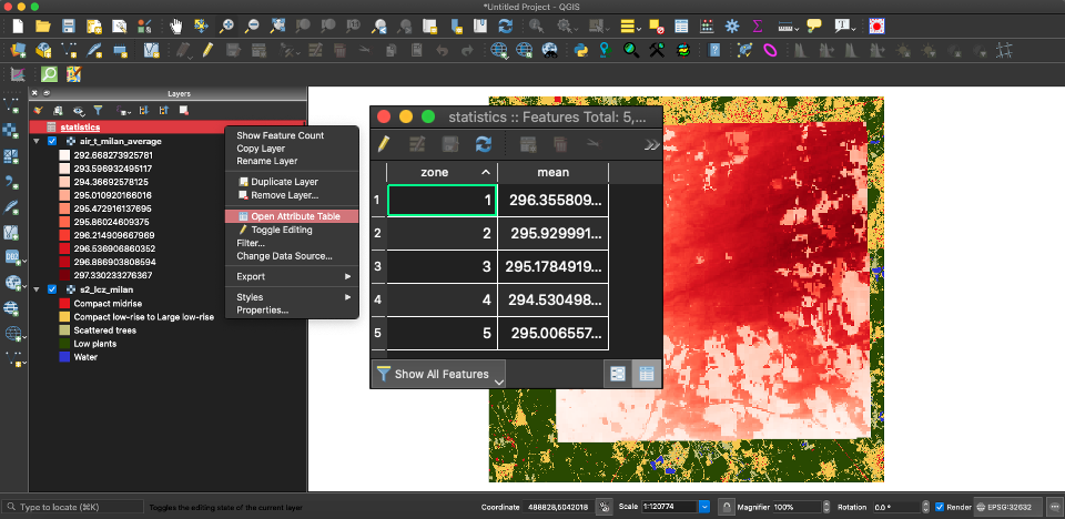
The output file contains the summary statistics by LCZ class computed for the average air temperature raster. No geometries are included in the output.”

Open, explore and comment the output table by focusing on the columns zone (i.e. LCZ class) and mean (i.e. average air temperature).

Results¶

It is possible now to plot the resulting table using e.g. the Data Plotly QGIS plugin. From the QGIS menu, open: Plugin –> Manage and Install Plugins, search for Data Plotly plugin and install it.

The difference of average air temperature in each LCZ class can be appreciated e.g. by plotting the columns zone (X-axis) and mean (Y-axis) using a Scatter Plot.

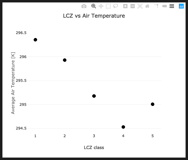
Results visualization by means of a Scatter Plot

Can we observe and quantify differences in the average air temperature within different LCZ of a city?

The answer is “Yes, we can measure these differences that are around 2 Kelvin degrees between heavily urbanized areas (1 = Compact midrise) and vegetated areas (4 = Low plants) for this case study”

[4]	Loftian, M. (2016). Urban climate modeling: case study of Milan city. Politecnico di Milano (M.Sc. dissertation).

[5]	Oxoli, D., Ronchetti, G., Minghini, M., Molinari, M. E., Lotfian, M., Sona, G., & Brovelli, M. A. (2018). Measuring urban land cover influence on air temperature through multiple geo-data—The case of Milan, Italy. ISPRS International Journal of Geo-Information, 7(11), 421.